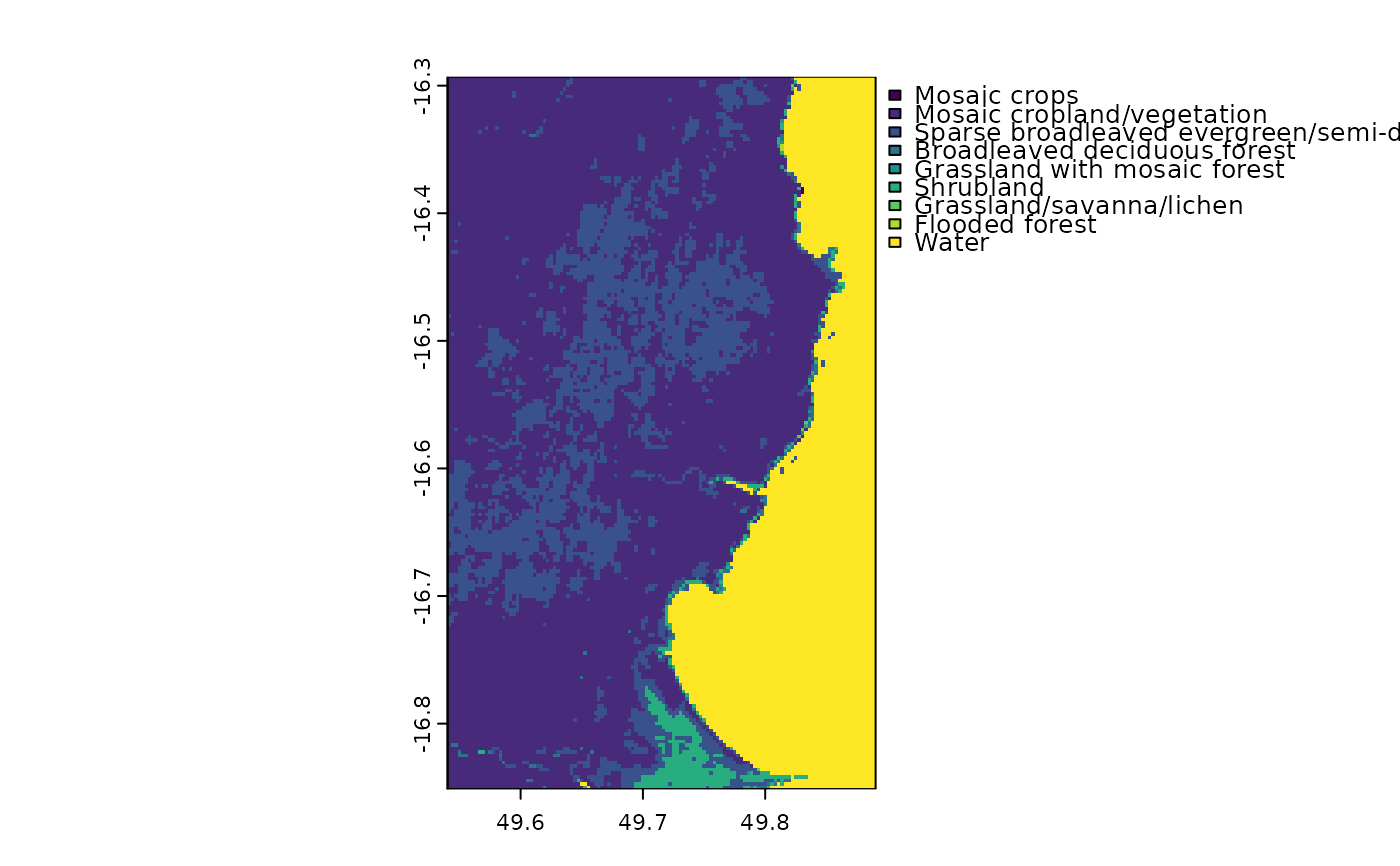
Table of land cover classes for an eastern portion of Madagascar
Source:R/madCoverCats.r
madCoverCats.RdThis data frame corresponds to the madCover raster, which represents land cover for an eastern portion of Madagascar. Note that the land cover classes have been simplified, so this table and raster should not be used for "real" analyses.
References
Arino O., P. Bicheron, F. Achard, J. Latham, R. Witt and J.-L. Weber. 2008. GlobCover: The most detailed portrait of Earth. European Space Agency Bulletin 136:25-31. http://due.esrin.esa.int.
Examples
### vector data
library(sf)
# For vector data, we can use data(*) or fastData(*):
data(madCoast0) # same as next line
madCoast0 <- fastData("madCoast0") # same as previous
madCoast0
#> Simple feature collection with 1 feature and 3 fields
#> Geometry type: MULTIPOLYGON
#> Dimension: XY
#> Bounding box: xmin: 2524653 ymin: -1767812 xmax: 2560090 ymax: -1709191
#> Projected CRS: Africa_Lambert_Conformal_Conic
#> COUNTRY NAME_1 NAME_2 geometry
#> 1 Madagascar Toamasina Analanjirofo MULTIPOLYGON (((2524653 -17...
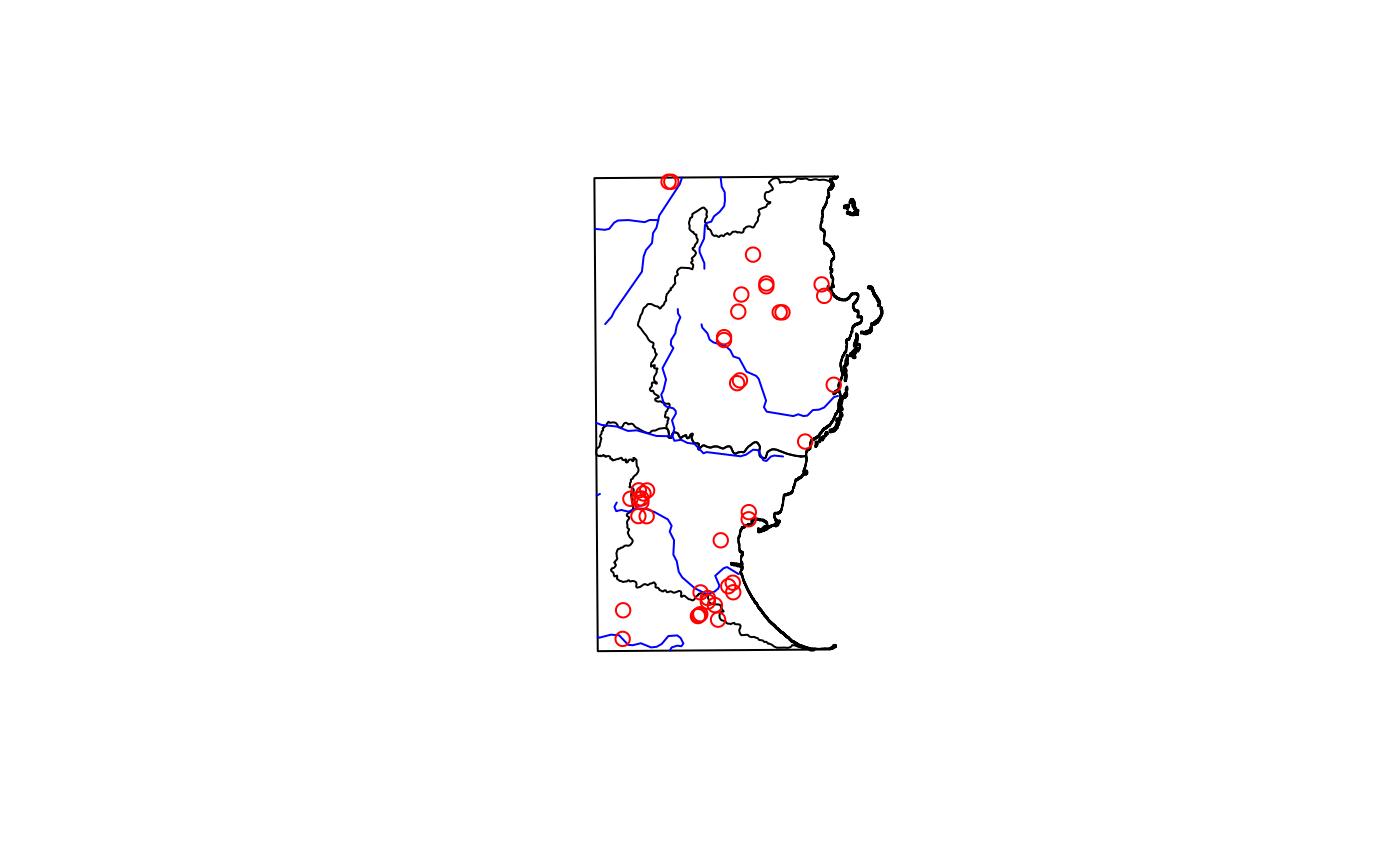
plot(st_geometry(madCoast0))
madCoast4 <- fastData("madCoast4")
madCoast4
#> Simple feature collection with 2 features and 5 fields
#> Geometry type: MULTIPOLYGON
#> Dimension: XY
#> Bounding box: xmin: 2524653 ymin: -1767812 xmax: 2560140 ymax: -1709141
#> Projected CRS: Africa_Lambert_Conformal_Conic
#> COUNTRY NAME_1 NAME_2 NAME_3 NAME_4
#> 1 Madagascar Toamasina Analanjirofo Mananara Antanambe
#> 2 Madagascar Toamasina Analanjirofo Soanierana-Ivongo Manompana
#> geometry
#> 1 MULTIPOLYGON (((2558667 -17...
#> 2 MULTIPOLYGON (((2533558 -17...
plot(st_geometry(madCoast4), add = TRUE)
madRivers <- fastData("madRivers")
madRivers
#> Simple feature collection with 3 features and 3 fields
#> Geometry type: LINESTRING
#> Dimension: XY
#> Bounding box: xmin: 2524653 ymin: -1767812 xmax: 2550723 ymax: -1709191
#> Projected CRS: Africa_Lambert_Conformal_Conic
#> TopElev BotElev Slope geometry
#> 1 495 2 0.005781444 LINESTRING (2524653 -173852...
#> 2 652 4 0.005808253 LINESTRING (2524653 -171484...
#> 3 24 0 0.001063664 LINESTRING (2524653 -176531...
plot(st_geometry(madRivers), col = "blue", add = TRUE)
madDypsis <- fastData("madDypsis")
madDypsis
#> Simple feature collection with 13 features and 13 fields
#> Geometry type: POINT
#> Dimension: XY
#> Bounding box: xmin: 2513925 ymin: -1763063 xmax: 2550698 ymax: -1718803
#> Projected CRS: Africa_Lambert_Conformal_Conic
#> First 10 features:
#> gbifID species country stateProvince latitude longitude
#> 1 1258262878 Dypsis boiviniana Madagascar Toamasina -16.50000 49.80000
#> 2 1258261855 Dypsis forficifolia Madagascar Toamasina -16.50000 49.72000
#> 3 4031635203 Dypsis faneva Madagascar Toamasina -16.43333 49.44166
#> 4 4032077789 Dypsis fanjana Madagascar Toamasina -16.45000 49.76667
#> 5 1258261866 Dypsis paludosa Madagascar Toamasina -16.45000 49.76666
#> 6 4032047806 Dypsis ramentacea Madagascar Toamasina -16.41667 49.75000
#> 7 4032124261 Dypsis fasciculata Madagascar Toamasina -16.38333 49.73333
#> 8 4031363900 Dypsis paludosa Madagascar Toamasina -16.53333 49.71667
#> 9 4032132562 Dypsis pinnatifrons Madagascar Toamasina -16.77694 49.71611
#> 10 4032072554 Dypsis heterophylla Madagascar Toamasina -16.78416 49.68555
#> day month year institution license rightsHolder
#> 1 16 4 1992 Missouri Botanical Garden CC_BY_4_0 Missouri Botanical Garden
#> 2 NA NA NA Missouri Botanical Garden CC_BY_4_0 Missouri Botanical Garden
#> 3 NA 10 1991 Missouri Botanical Garden CC_BY_4_0 Missouri Botanical Garden
#> 4 5 10 1991 Missouri Botanical Garden CC_BY_4_0 Missouri Botanical Garden
#> 5 21 4 1992 Missouri Botanical Garden CC_BY_4_0 Missouri Botanical Garden
#> 6 7 10 1991 Missouri Botanical Garden CC_BY_4_0 Missouri Botanical Garden
#> 7 NA 4 1992 Missouri Botanical Garden CC_BY_4_0 Missouri Botanical Garden
#> 8 26 2 1987 Missouri Botanical Garden CC_BY_4_0 Missouri Botanical Garden
#> 9 29 6 2007 Missouri Botanical Garden CC_BY_4_0 Missouri Botanical Garden
#> 10 4 7 2007 Missouri Botanical Garden CC_BY_4_0 Missouri Botanical Garden
#> recordedBy geometry
#> 1 H.J. Beentje;al. POINT (2550698 -1731317)
#> 2 POINT (2542470 -1731222)
#> 3 H.J. Beentje POINT (2513925 -1723786)
#> 4 H.J. Beentje POINT (2547331 -1725948)
#> 5 H.J. Beentje;al. POINT (2547331 -1725948)
#> 6 H.J. Beentje POINT (2545658 -1722375)
#> 7 H.J. Beentje;John Dransfield POINT (2543985 -1718803)
#> 8 Marion F. Nicoll POINT (2542086 -1734771)
#> 9 Adolphe Lehavana;al. POINT (2541728 -1760759)
#> 10 Honoré Andriamiarinoro POINT (2538576 -1761493)
plot(st_geometry(madDypsis), col = "red", add = TRUE)
 ### raster data
library(terra)
# For raster data, we can get the file directly or using fastData(*):
rastFile <- system.file("extdata/madElev.tif", package="fasterRaster")
madElev <- terra::rast(rastFile)
madElev <- fastData("madElev") # same as previous two lines
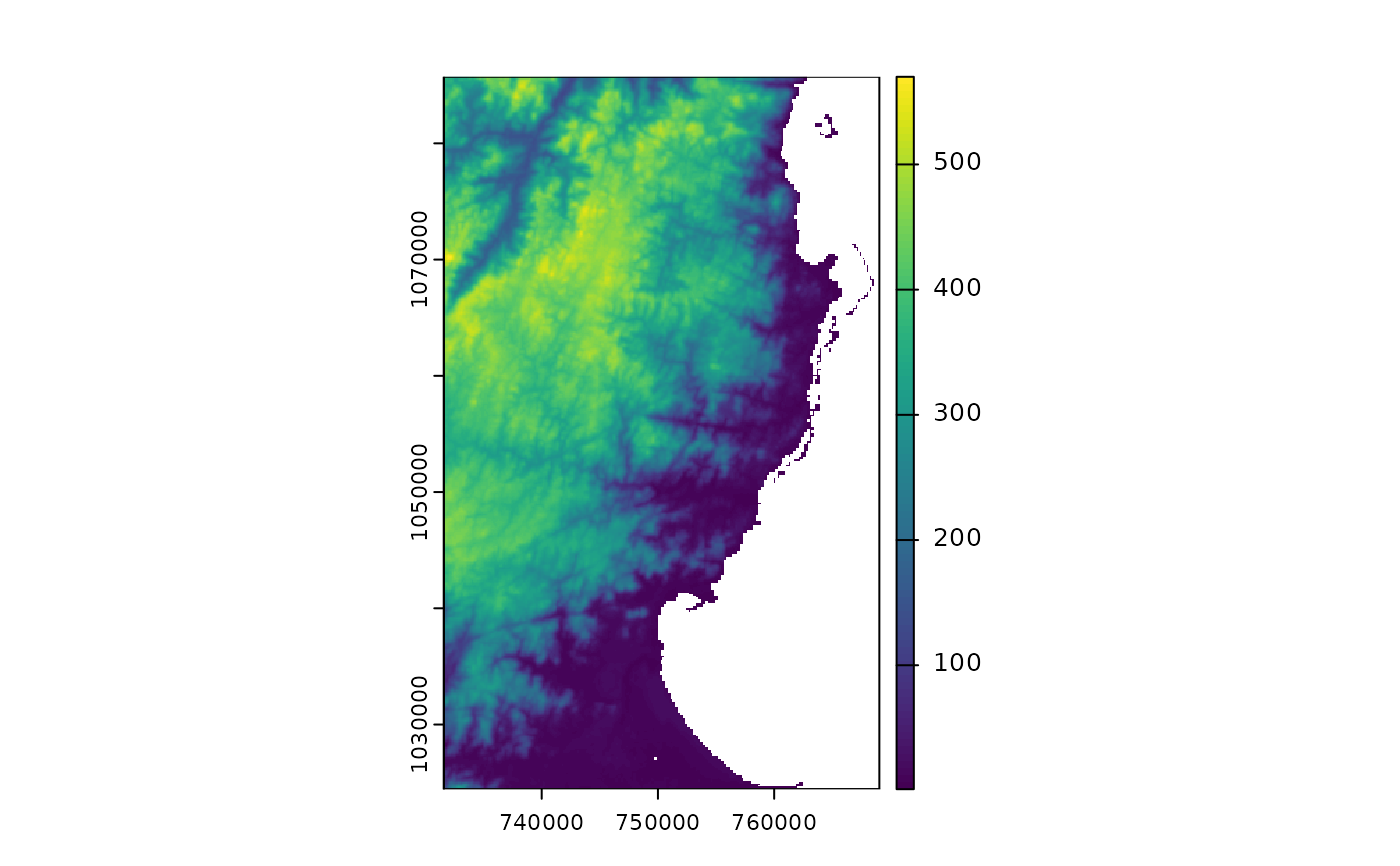
madElev
#> class : SpatRaster
#> size : 1090, 667, 1 (nrow, ncol, nlyr)
#> resolution : 54.99431, 54.99431 (x, y)
#> extent : 2523700, 2560381, -1768756, -1708812 (xmin, xmax, ymin, ymax)
#> coord. ref. : Africa_Lambert_Conformal_Conic
#> source : madElev.tif
#> name : madElev
#> min value : 4
#> max value : 520
plot(madElev)
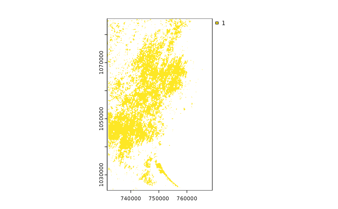
 madForest2000 <- fastData("madForest2000")
madForest2000
#> class : SpatRaster
#> size : 1090, 667, 1 (nrow, ncol, nlyr)
#> resolution : 54.99431, 54.99431 (x, y)
#> extent : 2523700, 2560381, -1768756, -1708812 (xmin, xmax, ymin, ymax)
#> coord. ref. : Africa_Lambert_Conformal_Conic
#> source : madForest2000.tif
#> name : madForest2000
#> min value : 1
#> max value : 1
plot(madForest2000)
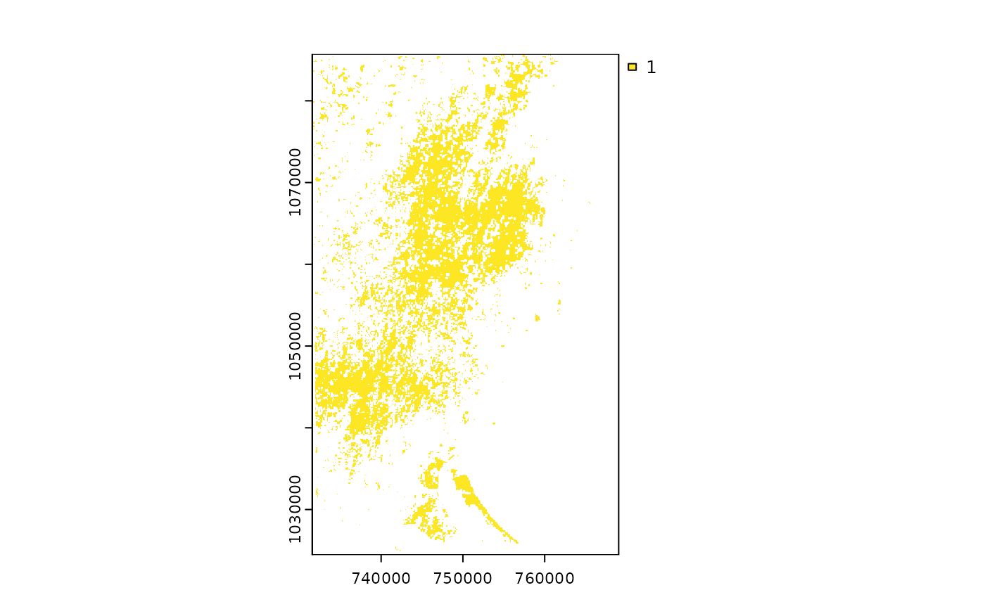
 madForest2014 <- fastData("madForest2014")
madForest2014
#> class : SpatRaster
#> size : 1090, 667, 1 (nrow, ncol, nlyr)
#> resolution : 54.99431, 54.99431 (x, y)
#> extent : 2523700, 2560381, -1768756, -1708812 (xmin, xmax, ymin, ymax)
#> coord. ref. : Africa_Lambert_Conformal_Conic
#> source : madForest2014.tif
#> name : madForest2014
#> min value : 1
#> max value : 1
plot(madForest2014)
 # multi-layer rasters
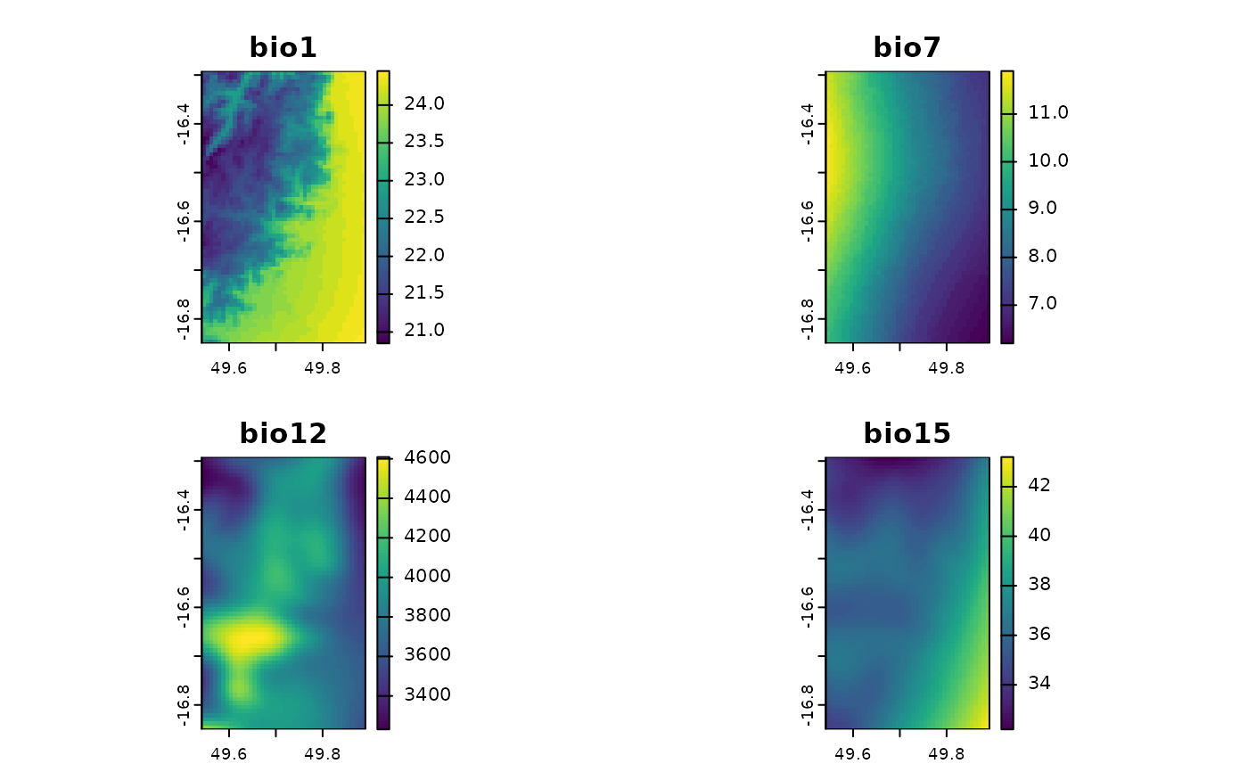
madChelsa <- fastData("madChelsa")
madChelsa
#> class : SpatRaster
#> size : 67, 42, 4 (nrow, ncol, nlyr)
#> resolution : 0.008333333, 0.008333333 (x, y)
#> extent : 49.54153, 49.89153, -16.85014, -16.29181 (xmin, xmax, ymin, ymax)
#> coord. ref. : lon/lat WGS 84 (EPSG:4326)
#> source : madChelsa.tif
#> names : bio1, bio7, bio12, bio15
#> min values : 20.85, 6.2, 3230.899902, 32.200001
#> max values : 24.450001, 11.9, 4608.899902, 43.200001
plot(madChelsa)
 madPpt <- fastData("madPpt")
madTmin <- fastData("madTmin")
madTmax <- fastData("madTmax")
madPpt
#> class : SpatRaster
#> size : 91, 65, 12 (nrow, ncol, nlyr)
#> resolution : 877.8452, 877.8452 (x, y)
#> extent : 2514147, 2571207, -1778842, -1698958 (xmin, xmax, ymin, ymax)
#> coord. ref. : Africa_Lambert_Conformal_Conic
#> source : madPpt.tif
#> names : ppt01, ppt02, ppt03, ppt04, ppt05, ppt06, ...
#> min values : 311, 421, 400, 289, 235, 229, ...
#> max values : 474, 591, 574, 492, 442, 409, ...
madTmin
#> class : SpatRaster
#> size : 91, 65, 12 (nrow, ncol, nlyr)
#> resolution : 877.8452, 877.8452 (x, y)
#> extent : 2514147, 2571207, -1778842, -1698958 (xmin, xmax, ymin, ymax)
#> coord. ref. : Africa_Lambert_Conformal_Conic
#> source : madTmin.tif
#> names : tmin01, tmin02, tmin03, tmin04, tmin05, tmin06, ...
#> min values : 20, 20, 20, 19, 18, 16, ...
#> max values : 25, 26, 25, 25, 24, 23, ...
madTmax
#> class : SpatRaster
#> size : 91, 65, 12 (nrow, ncol, nlyr)
#> resolution : 877.8452, 877.8452 (x, y)
#> extent : 2514147, 2571207, -1778842, -1698958 (xmin, xmax, ymin, ymax)
#> coord. ref. : Africa_Lambert_Conformal_Conic
#> source : madTmax.tif
#> names : tmax01, tmax02, tmax03, tmax04, tmax05, tmax06, ...
#> min values : 26, 26, 25, 24, 23, 21, ...
#> max values : 29, 29, 28, 27, 26, 24, ...
# RGB raster
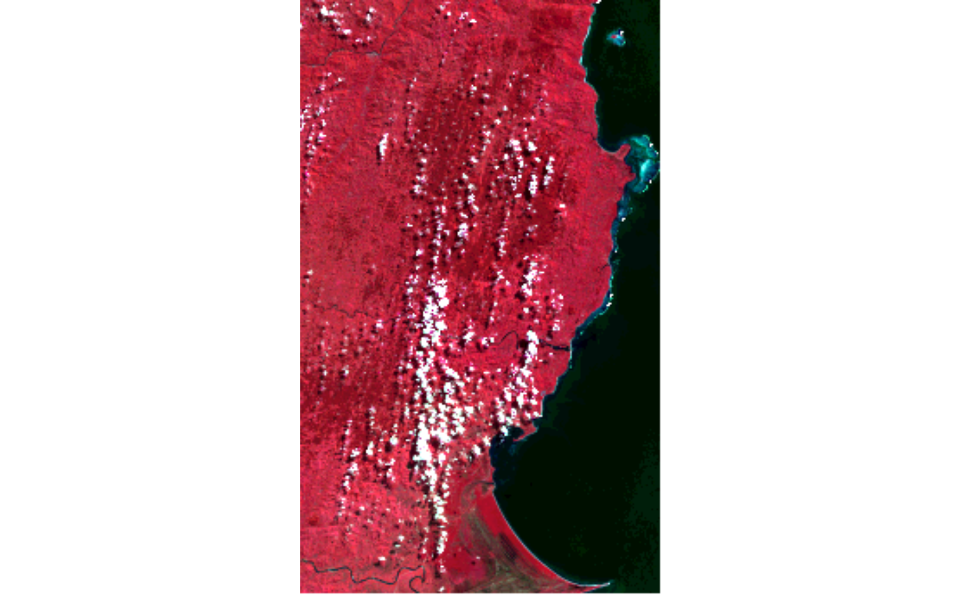
madLANDSAT <- fastData("madLANDSAT")
madLANDSAT
#> class : SpatRaster
#> size : 344, 209, 4 (nrow, ncol, nlyr)
#> resolution : 180, 180 (x, y)
#> extent : 344055, 381675, -1863345, -1801425 (xmin, xmax, ymin, ymax)
#> coord. ref. : WGS 84 / UTM zone 39N (EPSG:32639)
#> source : madLANDSAT.tif
#> names : band2, band3, band4, band5
#> min values : 15, 23, 22, 25
#> max values : 157, 154, 158, 166
plotRGB(madLANDSAT, 4, 1, 2, stretch = "lin")
 # categorical raster
madCover <- fastData("madCover")
madCover
#> class : SpatRaster
#> size : 201, 126, 1 (nrow, ncol, nlyr)
#> resolution : 0.002777778, 0.002777778 (x, y)
#> extent : 49.54028, 49.89028, -16.85139, -16.29306 (xmin, xmax, ymin, ymax)
#> coord. ref. : lon/lat WGS 84 (EPSG:4326)
#> source : madCover.tif
#> categories : Short, Long
#> name : Short
#> min value : Mosaic crops
#> max value : Water
madCover <- droplevels(madCover)
levels(madCover) # levels in the raster
#> [[1]]
#> Value Short
#> 1 20 Mosaic crops
#> 2 30 Mosaic cropland/vegetation
#> 3 40 Sparse broadleaved evergreen/semi-deciduous forest
#> 4 50 Broadleaved deciduous forest
#> 5 120 Grassland with mosaic forest
#> 6 130 Shrubland
#> 7 140 Grassland/savanna/lichen
#> 8 170 Flooded forest
#> 9 210 Water
#>
nlevels(madCover) # number of categories
#> [1] 0
catNames(madCover) # names of categories table
#> [[1]]
#> [1] "Value" "Short" "Long"
#>
plot(madCover)